
Shell.ai Hackathon for Sustainable and Affordable Energy

With growing population and rising demands leading to climate change, the planet is in need of a cleaner and smarter energy solution. Shell believes that AI can provide critical support to the energy sector in its transition from fossil-based energy solutions to a zero-carbon emission system. A lot is banking on wind energy and this hackathon, by Shell, is a step in the direction of a smarter energy transition drive.
Motivation
Optimal layout of wind turbines in a wind farm carries huge business importance with unoptimized or suboptimal layouts costing up to 5-15% of AEP (Annual Evergy Production). The key problem with an unoptimized layout is the combined influence of arranged wind turbines on the wind speed distribution across the limited area of the farm. As a wind turbine extracts energy from the incoming wind, it creates a region behind it, downstream, where the wind velocity is decreased - wake region. Due to the induced speed deficit, a turbine placed inside the wake region of an upstream turbine will naturally generate reduced electrical power, as is evident from Fig. 1. This inter-turbine interference is known as the wake effect. Thus, strategies for optimal wind turbine layout needs to be employed in order to keep power losses at a minimum.
Optimizing the layout of a wind farm is a complex optimization problem due to its high dimensionality, complex multimodality, and discontinuous nature of the search space. Hence, optimizing the layout analytically is difficult and requires AI based solutions.
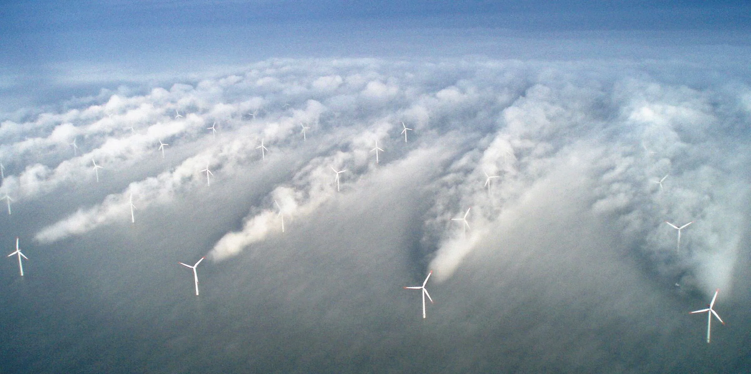
Fig. 1: The wake-effect in action. Turbines directly in the wake region of another turbine produce considerably less power.
Problem Statement
In this hackathon, the challenge was to optimize the placement of $50$ wind turbines of $100$m rotor diameter and $100$m height each on a hypothetical $4$km$\times4$km, 2D offshore wind farm area such that AEP (Annual Energy Production) of the farm is maximized. The orientation of the farm is such that the positive $x$ and $y$ axis are aligned with the geographical East and North directions, respectively. Also, the following two constraints cannot be violated at any given time
- Perimeter Constraint - All turbines must maintain a minimum clearance of $50$m from the farm boundary.
- Proximity Constraint - The distance between any two turbines must be at least $400$m.
We were provided with seven csv files containing approximately half-hourly wind data gathered from an anonymous location for seven different years. The organizers also provided us with code to generate AEP scores for obtained turbine positions.
An Initial Take
Before diving deep into the problem, we decided to simplify it in order to perform some quick, initial experiments so as to get a feel of the problem statement. Since the major constraint which we need to consider is that of proximity, we decided to bake this constraint right into the solution itself. The total available space is $3950-50=3900$m with each turbine requiring a minimum safe distance of $400$m. Based on this fact, we transform the search space into a discrete problem by considering only $3900/400\approx9$ boxes in both $x$ and $y$ axes resulting in a total of 81 boxes. Thus, the problem is simplified into placing 50 turbines in 81 boxes such that AEP is maximized. To experiment with this idea, we decided to use off-the-shelf algorithms, namely the Genetic Algorithm (GA) as it is easy and intuitive to code.
Instead of starting the GA on a random state, we run 1000 iterations with each iteration randomly placing 50 turbines in the discrete space (refer to Fig. 2). The configuration with maximum AEP score is selected as the start state for the genetic algorithm.

Fig. 2: $9\times9$ search space with $50$ turbines being placed randomly to get a good start state.

Fig. 3: The final, best solution provided by GA for the discrete version of windfarm layout.
GA's performance tapered off at an approximate AEP score of 532, putting us at the 154th spot on the leaderboard. Fig. 3 is the resulting configuration with corresponding code made available below. From this small and quick experiment, we realized two things. Firstly, we need to work on the continuous space as a discrete version of the problem ignores a huge number of possible states. In other words, it only considers a very small portion of the entire search space. Secondly, in order to learn, enjoy and truly gain experience from the competition, we decided to come up with our very own optimization algorithm! (It isn't that hard, trust me)
Code for optimizing the discrete space version of the windfarm layout using GA.
A New Approach
Having gone back to the drawing board, the first thing we did was to analyze the data by plotting a wind rose chart. Fig. 4 (wind rose chart) shows the average wind speed distribution over seven years. Looking at the chart and reading related literature, we realized that the best possible layout would be the one packing maximum turbines at the edges of the windfarm.

Fig. 4: Wind rose chart describing the average wind speed distribution over 7 years
Generating an initial windfarm layout by hand without any visual aid is quite painstaking. At the same time, having some sort of interactive tool that would, in realtime, output an AEP score for any change to the windfarm layout would be really handy. Therefore, we developed a small, interactive application in python that allows users to visually select and move turbines while the corresponding AEP score of the resulting windfarm layout is provided as output. Vid. 1 shows this tool in action. Corresponding code for the entire tool is also provided.
Using the application, we directly place $10+8+10+8=36$ turbines corresponding to the top, left, bottom and right edges, respectively. These are the maximum number of turbines that can be packed at the edges. The remaining 14 turbines are randomly placed. This forms our intial layout. Now all that is required is an algorithm to optimize our layout.
Entire code for generating an interactive, realtime editor for windfarm layouts, as demonstrated in the video above
The algorithm - NDOpt
Let us consider a discrete version of the windfarm layout optimisation problem and try to draw some parallel with the $N$-Queens problem. The $N$-Queens problem requires placement of $N$ queen pieces on a $N \times N$ chessboard such that no two queens can attack each other. In a similar vein, the windfarm layout optimisation problem requires placement of $50$ turbines on a $9\times9$ grid. But there are two major dissimilarities here. Unlike the $N$-Queens problem, a valid placement configuration does not translate to the best possible solution. Also, as stated earlier, a discrete version of our problem is limiting while the search space on a continuous version is for all intents and purposes, infinite. Therefore, no backtracking (and consequently no dynamic programming) can be applied to solve our problem, which is typically the algorithm of choice for $N$-Queens. Based on these observations, we realized that a greedy algorithm was the way to go.
Having understood, the type of algorithm required, we moved on to actually developing one. Again, let us consider how a neural network learns. In essence, it changes its weights by some amount (learning rate) based on some error in the direction of the best score. Since we are working on an optimization setting, we can forego of the error part. Remember that we have a model, provided by the organizers, that can output an AEP score given a layout. This takes care of the scoring part of our algorithm. Since we have already determined that a greedy algorithm is required, we can therefore consider a single turbine at a time. As the turbines are on a 2D space, we can assume 8 possible directions of movement. Moving a turbine by some amount in each direction and evaluating the result gives us 8 different scores. We can then update the current turbine position (weight) by an amount specified by the learning rate in the direction of local optima. Thus, we have successfully developed a greedy optimization algorithm which embodies the essence of the working principle of a neural network! Fig. 5 is a visualization of our algorithm's core concept.

Fig. 5: Visualization of the core concept of our proposed algorithm, NDOpt (Non-differentiable Optimisation)
Additions and Improvements
What has been described above is simply the core idea. We added a lot of other features and improved upon the core concept. The following section gives a step-by-step account of how we improved our approach.
Fixing proximity constraint
As you might have understood, moving a turbine individually may violate the proximity constraint with other turbines. Up till now, we were simply discarding the states which produced these violations. But such states can contribute to a better score if the violations are fixed.
NDOpt does not require a differentiable cost function which makes it easy to implement for different optimisation problems. We reimplemented NDOpt but changed the cost function to output the minimum distance of current turbine with all other turbines instead of an AEP score. In this case, the best direction to move becomes the direction which leads to an increase in the minimum distance until all turbines are at least $400$m apart. This results in an algorithm that can fix any constraint violating layout. All of the consequent improvements and additions to NDOpt also applies to this algorithm.
Shuffling
NDOpt updates the position of each turbine, individually at each iteration. We realized that the turbines updated before others receive higher priority with the very first turbine practically deciding the course of traversal through the search space. This is because once a turbine's position is updated, the next turbine's local optima is calculated with respect to the previous updation. This causes our algorithm to traverse only a subset of the search space which is not ideal. Therefore, after each iteration, the turbines are shuffled so that the sequence of updation changes.
Variable learning rate
This is a pretty straightforward improvement. Once the direction for the best position is found, instead of moving a turbine by learning rate in this direction, multiple different learning rates are tried out and the one which gives maximum AEP is selected. Therefore, each turbine, at any given epoch, moves by a different learning rate. This feature drastically improved our convergence time.
Increased degrees of freedom
Earlier, we stated that one can assume 8 directions of movement in 2D space. This assumption is wrong since an object can move in any of the 360 degrees on a 2D plane. But not all directions are important since change by one degree offers nearly the same AEP score. We therefore consider 36 directions, one at every 10 degrees. In case you are wondering how to generate a direction vector, remember that a unit vector gives us the direction and multiplying it with a scalar provides us with a new position. This unit vector can be calculated as $$x=\cos(\theta)$$ $$y=\sin(\theta)$$ where $x$ and $y$ are the values of the respective axes.
Noise to escape local maxima
Every optimisation algorithm traversing a search space looking for that elusive global optima will encounter local optimas and possibly get stuck in them. NDOpt is no exception to the case. In order to deal with this, we added some noise to the learning rate. The value of the noise variable remains zero when the algorithm is not stuck at a local optima but when it does get stuck, a counter is increamented by one and this counter exponentially scales the noise. Every iteration that the algorithm is stuck at a local optima, the value of the noise variable increases and as soon as the algorithm escapes the area, the value of the counter is set back to zero and so is the value of the noise variable. The idea is that, taking a large step instead of small ones will cause the algorithm to jump out of its current predicament and land far away from the local optima. This might result in a temporary reduction in AEP but the algorithm will be able to traverse the search space better and soon improve upon its previous score.
Ensemble
Having competed in multiple hackathons, we cannot shake off the urge to finish off our solution without performing some sort of ensembling. Ensembling basically means to combine two or more solutions such that the resulting solution is better than both. In order to get two different solutions, we ran two separate versions of NDOpt. The former updates the positions of all turbines while the latter updates the position of only the interior turbines. Once both the solutions reached their maximum possible AEP score, they were combined together to yield our final result.
Our ensembling technique is really simple. Assume that we have two solutions, 1 and 2 such that AEP score of solution 1 is greater than that of solution 2. A turbine in solution 1 is replaced by the turbine from solution 2 with which it has minimum distance. The resulting layout's AEP score is calculated and if the score is higher than both solutions 1 and 2, then the new position of the current turbine is fixed in solution 1. This happens for each turbine. Finally, the new, updated solution 1 is presented as our final windfarm layout. This ensembling technique improved our results and provided us with a jump on the leaderboard.

Fig 6: Ensembling visualisation of windfarm layout optimization problem.
Conclusion
Integrating all of the above ideas together, into a single algorithm, NDOpt, got our team, deepwizAI.com, comprising of Atif Hassan, Sayantan Basu and Gourab Chowdhury shortlisted as the top 10 teams in the Student Edition of the Shell.ai hackathon with the final winners being declared on November 12th, 2020. We reached the top spot in just under 8 days compared to one month available for others. This was one of the best hackathons we have ever participated in. Thank you so much Shell!

Fig 7: The graph depicts our progress on the public leaderboard. 1 indicates the Genetic Algorithm phase. 2 indicates the progress made by implementing NDOpt algorithm. 3 indicates the final phase of our solution when we applied our new ensembling technique.