How to correctly use TF-IDF with imbalanced data

a single shark as minority taking on a majority of fishes

If you have been employing TF-IDF with imbalanced data while setting some hyper-parameter which limits the number of features used, then you are probably hurting your Machine Learning (ML) model’s performance by supplying an incorrect feature-set. In this article, I will show you a nifty trick that can get you back on track!

Note: Throughout this blog post, it is assumed that you are using the scikit-learn implementation of TF-IDF $^{[1]}$ .

TF-IDF: An overview

TF-IDF stands for Term Frequency Inverse Document Frequency. To put it simply, TF-IDF returns a number (a scalar value) for every word that we have in a corpus (a set of documents) which denotes how important that given word is. It calculates this number/statistic using the following formula, $\text{tfidf}(x,y) = \text{tf}(x,y) \times log \left( \frac{N}{\text{df}(x)} \right)$ where, $x$ is a word, $y$ is a document, $\text{tf}(x, y)$ is the frequency of word $x$ in document $y$ , $N$ is the total number of documents and $\text{df}(x)$ is the number of documents containing the word $x$ . Finally, $\text{tfidf}$ is the TF-IDF score for word $x$ in document $y$ .

Here, the first term in the equation refers to term frequency while the second term refers to inverse document frequency. The two terms are exactly opposite in the way they assign importance to words.

Problem with Vanilla TF-IDF

It is very natural to limit the number of features representing a single document. This can be done by using either of the min_df, max_df or max_features hyper-parameters. For now, let us focus on max_features. The same logic will follow for the other two hyper-parameters as well.

The purpose of max_features is to limit the number of features (words) from the dataset for which we want to calculate the TF-IDF scores. This is done by choosing the features based on term frequency across the corpus $^{[1]}$ .

Why is this a problem? Consider you are working with the IMDB dataset and you need to predict whether a review is positive or negative. Assume that you sub-sampled the dataset in such a way that you ended up with $23$ K negative reviews and $2$ K positive reviews. Now if you run TF-IDF on top of this, with some value of max_features, there is a high chance that the majority of words chosen will be from the majority class (negative words/features). This makes sense since TF-IDF is selecting features based on term frequency alone and negative words are present in most of the samples. As a result, the minority class gets under-represented. This is demonstrated in Fig. 1, wherein it is clear that only after setting the max_features hyper-parameter to a really large value are the positive words selected as features by TF-IDF. This is not desirable as more features would require more samples, leading to curse of dimensionality.

Note: When creating Fig. 1, common words were excluded from the counting process.

Fig.1: As the max_features hyper-parameter is increased, no positive words/features are added into the feature-set until a very large value is reached

Intuition

We have now understood that TF-IDF does not correctly represent minority class words because it chooses features based on term frequency alone. So what can we do to ensure that we pick words from the minority class?

The first step is to understand that word frequencies between minority class and majority class are not comparable as majority class words will have a much higher frequency than the minority class. Thus, to represent both, we have to isolate the classes and then pick out the words. This way we ensure that we are selecting words from both majority and minority classes.

The next step will be to decide how many features we want to select. Let us say that we want a total of $300$ features (max_features= $300$ ). Out of this $300$ how do we decide on the number features that should be attributed to the majority and minority classes? We can take $150$ features per class but this will lead to under-representation of the majority class. Thus, some sort of weighting mechanism is required.

Solution: Weighted Class TF-IDF

Let us consider the following example. Assume there exists a dataset having two labels $0$ and $1$ with class $0$ containing $80\%$ of the samples while class $1$ containing the remaining $20\%$ . Also, assume that max_features= $300$ . At first, we calculate the weight for each label. Weight here refers to the number of features that should be selected from each class. Since class $0$ is present in $80\%$ of the records, we will pick $240$ features from class $0$ and $60$ features from class $1$ . These values can be calculated based on the following formula, $f_{c_i} = \text{max_features} \times \frac{n_{c_i}}{n_d}$

Here, $n_{c_i}$ is the number of samples in the $i$ -th class, $n_d$ is the total number of samples and $f_{c_i}$ is the number of features to be selected for the $i$ -th class.

Now we run TF-IDF separately on class $0$ and class $1$ with max features set to $240$ and $60$ , respectively. Further, in order to ensure non-overlapping feature-set between both classes, features selected in class $0$ are passed as stop-words to the stop_words hyperparameter when running TF-IDF over class $1$ .

Once complete, we combine the vocabulary from both classes into a single list. This can be easily achieved since TF-IDF provides a vocabulary_ parameter that stores the entire vocabulary.

Finally, this combined vocabulary is used as the fixed vocabulary in another TF-IDF model which runs over the entire data. By fixing the vocabulary for the final TF-IDF run, we ensure that all documents/samples are represented by these words/features only.

This entire, novel process is called Weighted Class TF-IDF or WCTF-IDF. Thus, to put it simply the $300$ features chosen by WCTF-IDF are a better representation of the overall data as compared to the features chosen by the vanilla TF-IDF model. I shall prove this via empirical results.

Code

The code available here is to show the performance of WCTF-IDF on a single dataset. Results have been reported on other datasets as well.

	import re
	import os
	import sys
	import warnings
	import pandas as pd
	from sklearn.feature_extraction.text import TfidfVectorizer
	from sklearn.model_selection import train_test_split
	from sklearn.metrics import classification_report
	from sklearn.linear_model import LogisticRegression
	from wcbtfidf import Wcbtfidf

	warnings.filterwarnings("ignore")


	def set_session_path():
	"""
	Set session path to current working directory
	"""
	module_path = os.path.abspath(os.path.join("../.."))
	if module_path not in sys.path:
	sys.path.append(module_path)


	def read_and_prepare_data(filename):
	"""
	Sample the dataset in an imbalancd way
	Compare imbalance statistics
	"""
	df = pd.read_csv(filename)

	print(f"Shape of the original dataset is {df.shape}")
	print(
	f"Target distribution of the original dataset \n{df.sentiment.value_counts(normalize=True)}"
	)

	df["sentiment"] = df["sentiment"].map({"negative": 0, "positive": 1})

	# Sampling data with imbalance
	# Total sample: 25k points
	# 23k points -> class 0
	# 2k points -> class 1

	negative_samples = df[df["sentiment"] == 0].sample(n=23000, random_state=60)
	positive_samples = df[df["sentiment"] == 1].sample(n=2000, random_state=60)

	# Merge and shuffle the imbalanced data
	final_df = pd.concat([negative_samples, positive_samples]).sample(
	frac=1, random_state=60
	)

	print(f"Final data shape is {final_df.shape}")
	print(
	f"Final target distribution is \n{final_df.sentiment.value_counts(normalize=True)}"
	)
	return final_df


	def preprocess_text(text):
	"""
	Sanitize input
	"""
	text = text.lower()
	text = re.sub("[^a-z0-9]", " ", text)
	text = re.sub("(\s)+", " ", text)
	return text


	def get_model(xtrain, xtest, ytrain, ytest, max_feat, model, type_model):
	"""
	Run model on imbalanced dataset
	"""
	if type_model == "TFIDF":
	print("Running TFIDF")
	tfidf = TfidfVectorizer(max_features=max_feat, stop_words="english")
	train_df = pd.DataFrame(
	tfidf.fit_transform(xtrain).toarray(), columns=tfidf.vocabulary_
	)
	test_df = pd.DataFrame(
	tfidf.transform(xtest).toarray(), columns=tfidf.vocabulary_
	)

	model.fit(train_df, ytrain)
	preds_tfidf = model.predict(test_df)
	print(classification_report(ytest, preds_tfidf))

	return tfidf

	if type_model == "WCBTFIDF":
	print("Running WCBTFIDF")
	wcbtfidf = Wcbtfidf(max_features=max_feat)
	wcbtfidf.fit(xtrain, ytrain)

	train_df = wcbtfidf.transform(xtrain)
	test_df = wcbtfidf.transform(xtest)

	model.fit(train_df, ytrain)
	preds_wcbtfidf = model.predict(test_df)
	print(classification_report(ytest, preds_wcbtfidf))

	return wcbtfidf


	def check_hypothesis(xtrain, xtest, ytrain, ytest, max_feat, model):
	"""
	Evaluate and return model objects
	"""

	tfidf = get_model(xtrain, xtest, ytrain, ytest, max_feat, model, "TFIDF")

	wcbtfidf = get_model(xtrain, xtest, ytrain, ytest, max_feat, model, "WCBTFIDF")

	return wcbtfidf, tfidf


	def analysis(wcbtfidf_object, tfidf_object):
	"""
	Vocab comparision statistics
	"""

	# Length Comparison

	tfidf_vocab = tfidf_object.vocabulary_
	wcbtfidf_vocab = wcbtfidf_object.combine_vocab

	print(len(wcbtfidf_vocab), len(tfidf_vocab))

	# Words that are present in tfidf vocab but not in wcbtfidf

	print(list(set(tfidf_vocab) - set(wcbtfidf_vocab)))

	# Words that are present in wcbtfidf but not in tfidf

	print(list(set(wcbtfidf_vocab) - set(tfidf_vocab)))


	def main():

	set_session_path()

	final_df = read_and_prepare_data("imdb_dataset.csv")
	final_df["clean_text"] = final_df["review"].apply(preprocess_text)

	final_df = final_df[["clean_text", "sentiment"]]
	xtrain, xtest, ytrain, ytest = train_test_split(
	final_df["clean_text"],
	final_df["sentiment"],
	test_size=0.25,
	random_state=60,
	stratify=final_df["sentiment"],
	)

	print(xtrain.shape, ytrain.shape)
	print(xtest.shape, ytest.shape)

	model = LogisticRegression()
	wcbtfidf_object, tfidf_object = check_hypothesis(
	xtrain, xtest, ytrain, ytest, 300, model
	)

	analysis(wcbtfidf_object, tfidf_object)


	if __name__ == "__main__":
	main()

view raw blog.py hosted with ❤ by GitHub

Results

In this section, I have provided exhaustive empirical results to demonstrate the effectiveness of WCTF-IDF against TF-IDF in an imbalanced data setting. On average, WCTF-IDF outperforms TF-IDF by $4\%$ under the F1-score metric.

Dataset	Class	Method	Precision	Recall	F1-Score	# samples
IMDB^[2]	0	TF-IDF	0.93	1.0	0.96	5750
	0	WCTF-IDF	0.93	0.99	0.96	5750
	1	TF-IDF	0.74	0.15	0.25	500
	1	WCTF-IDF	0.75	0.19	0.31	500

Table 1: 25K negative reviews and 2K positive reviews were selected to generate an imbalanced version of the IMDB dataset. Best values are denoted in bold. WCTF-IDF clearly outperforms TF-IDF on all metrics for the minority class while achieving the same performance on the majority class.

Dataset	Class	Method	Precision	Recall	F1-Score	# samples
Toxicity ^[3] Prediction	0	TF-IDF	0.93	1.0	0.96	35837
	0	WCTF-IDF	0.94	1.0	0.97	35837
	1	TF-IDF	0.93	0.36	0.52	4056
	1	WCTF-IDF	0.92	0.49	0.64	4056

Table 2: Toxicity Prediction is a multilabel classification dataset. This was converted to a binary classification dataset by giving the label 1 to those samples having at least one of the following classes {toxic, severe_toxic, obscene, threat, insult, identity_hate}. Again it can be clearly understood that WCTF-IDF outperforms TF-IDF on all metrics for the minority class while achieving slightly better performance on the majority class as well. Best values are denoted in bold.

Dataset	Class	Method	Precision	Recall	F1-Score	# samples
Sentiment140^[4]	0	TF-IDF	0.6	0.09	0.16	12500
	0	WCTF-IDF	0.61	0.12	0.2	12500
	1	TF-IDF	0.91	0.99	0.95	112500
	1	WCTF-IDF	0.91	0.99	0.95	112500

Table 3: WCTF-IDF once again outperforms TF-IDF on all metrics for the minority class while achieving same performance on the majority class. Best values are denoted in bold.

Ablation Study

Along with empirical results, I would also like to support my claim via in-depth analysis.

Running TF-IDF on the imbalanced version of the IMDB dataset and looking at the vocabulary list (note that only those words are being considered that appear in TF-IDF vocab but not in WCTF-IDF) shows that features are mostly composed of neutral or negative words such as {ridiculous, lack, cheap, ok, annoying, lost}. This makes sense because TF-IDF selects words simply on the basis of term frequency and a majority of the samples comprise of negative reviews. On the other hand, running WCTF-IDF results in mostly neutral or positive words (again, remember that only those words have been chosen that are present in WCTF-IDF vocab and not in TF-IDF) such as {loved, well, excellent, perfect, definitely, top, amazing, wonderful}. These positive words were not captured by the TF-IDF vocab as they were present in minority.

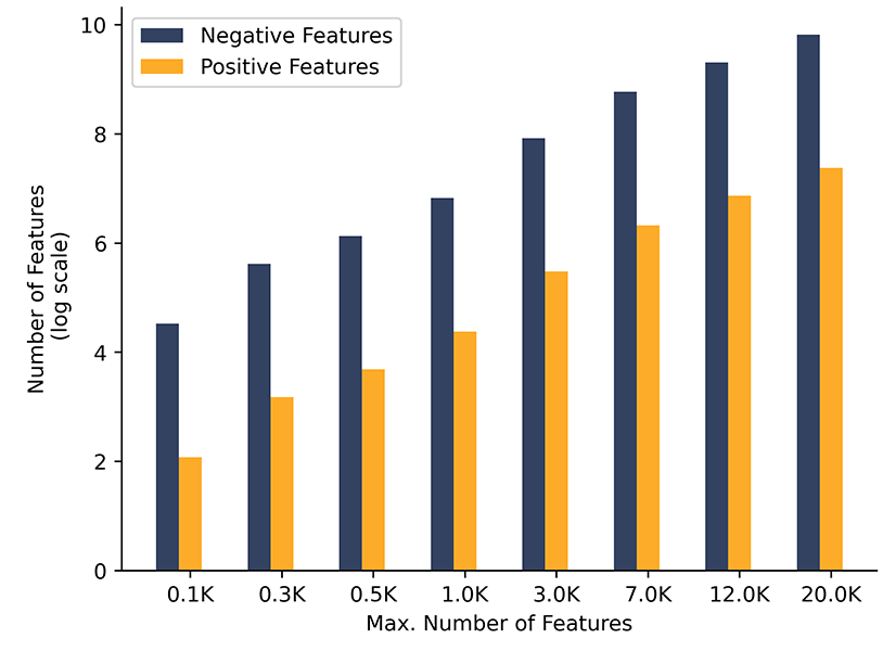
WCTF-IDF feature selection is representative of the imbalanced data

Fig. 2: As the max_features hyper-parameter is increased, WCTF-IDF selects the correct number of features in the minority class right from the start

Fig. 2 is in stark contrast to Fig. 1. Clearly, WCTF-IDF selects the representative number of features from the minority class while respecting the underlying class distribution. This is exactly what is required in an imbalanced data setting which further proves the efficacy of WCTF-IDF

Conclusion

Please find the link to the related GitHub repo here. The “demos” folder contains all of the remaining experiments in self-explanatory jupyter notebook files. Feel free to contribute to the repository if some enhancements and improvements can be made on the technique proposed above.

How to correctly use TF-IDF with imbalanced data

TF-IDF: An overview

Problem with Vanilla TF-IDF

Intuition

Solution: Weighted Class TF-IDF

Code

Results

Ablation Study

Conclusion

References

DeepwizAI

How to correctly use TF-IDF with imbalanced data

TF-IDF: An overview

Problem with Vanilla TF-IDF

Intuition

Solution: Weighted Class TF-IDF

Code

Results

Ablation Study

Conclusion

References

How to perform Unsupervised Feature Selection using Supervised Algorithms

An Unsupervised Neural Image Compression Algorithm

DeepwizAI